How to Create 3-D Drawings in Excel

How to Create 3-D Drawings in Excel

 

Microsoft Excel lets you add various kinds of shapes to make your spreadsheets look better. However, all of the shapes originally appear as flat 2-D drawings and that may not match any of the 3-D graphs or other objects that you may have on your spreadsheet. Create 3-D drawings in Excel by drawing any 2-D object on the worksheet and adjusting "3-D Format" and "3-D Rotation" properties.

Step 1

Click the "Insert" tab on the Microsoft Excel toolbar and click the "Shapes" button in the "Illustrations" group. Choose any of the shapes you want as the basis of your 3-D drawing.

Step 2

Click anywhere on the spreadsheet to create the shape with the normal properties. Click on the shape and use the "Format" tab on the toolbar to make any adjustments to the shape. For instance, you can choose one of the "Shape Styles" or adjust the "Shape Fill" or "Shape Outline" colors. Click on any of the small circles or boxes on the borders of the shape and drag them if you want to change the size of upcoming 3-D drawing.

Step 3

Right-click the shape and select "Format Shape" to bring up a dialog that lets you customize the shape even further. Click "3-D Rotation" from the left panel and click the box next to "Presets." Select any of the 3-D presets that closely matches your preference. If you need to make any additional adjustments, increase or decrease any of the X, Y, Z, or perspective values and see how they affect the shape.

Step 4

Click "3-D Format" from the left pane and increase the "Depth" value as high as you like. This reflects the thickness of your shape and will render the 3-D effect. Click the paint bucket next to "Color" in the "Depth" group to change the color of the third dimension. Click "Close" after you finished your edits.

Credit 

What Is Data Consolidation in Excel?

What Is Data Consolidation in Excel?

 

Microsoft Excel features a data-consolidation function that allows several tables to be consolidated into a single summary report. Consolidating the data often facilitates easier editing and viewing of information since it can be seen in aggregate form as a master spreadsheet. There are three basic ways to consolidate data in Excel: by position, category and formula. To locate the command, start by selecting the Data menu and then the Consolidate command, which will then prompt you to select one of the three consolidation options.

Consolidate by Position

The consolidate by position function works best when the data in the separate tables is consistent in position and arrangement. Using the consolidate by position function will move the contents from column A, for example, from all of the separate spreadsheets into a single spreadsheet. In addition, the aggregate consolidated spreadsheet can be set to automatically update when the data in the source spreadsheet changes.

Consolidate by Category

Consolidating by category allows spreadsheets with slightly different layouts, but consistent labels, to be consolidated into a master spreadsheet. The data will be extracted from the spreadsheet and organized automatically into the master spreadsheet. In order for this too to work properly, you must go into the "Insert" menu and define the label's name, and all spelling and capitalization must be identical for it to properly mesh.

Consolidate by Formula

Consolidation by formula uses a 3-D reference, which is a reference to a range that spans two or more worksheets in a workbook, to execute the consolidation. This method is most effective when you're working in a single Excel file with several worksheets. A cell contains a formula that references portions of another worksheet to be consolidate, which is effective when the worksheets are not identical in layout. If the worksheets are identical, then the worksheet name can be used as part of the consolidation formula.

Credit

How Do I Group Worksheets in Excel?

How Do I Group Worksheets in Excel?

 

A new file in Excel 2013 is called a workbook; the spreadsheet you work on is called a worksheet. By default, a workbook comes with one worksheet, although you can add more. The worksheets can be grouped together for simultaneous editing. After you make your edits, you can ungroup the worksheets to modify them individually.

 

Grouping Worksheets

Hold down the "Control" key while clicking specific worksheet tabs to group them. Spreadsheets that are linked together update at the same time. For example, if you group sheets 1 and 2 and type the word "test" in cell B2 on sheet 1, you can click over to sheet 2 and see the word "test" in the same cell. If you want to group multiple tabs in a row, select the tab for the first sheet you want to include in the group, hold the "Shift" key and click the last tab to group everything between the active tab and the one you click.

Ungrouping Excel Worksheets

When you're done with your edits, click a tab that isn't part of the group to disband the group. If every tab is linked, hold down the "Control" key and click any tab to deselect it from the group so it can be selected to ungroup the rest. Alternatively, right-click any grouped tab and select "Ungroup Sheets."

 

 

 

 

 

Credit 

How to Transfer Data From One Sheet to Another in Excel

 

How to Transfer Data From One Sheet to Another in Excel

 

Working with data in Microsoft Excel is not always easy to do. Formulas and functions can make even the simplest task seem challenging, even if, in reality, it isn't. Some people might use Excel at a very basic level: keeping all of their data on one sheet, not labeling columns or rows properly, or ignoring some settings (such as formatting) that can make data management much easier. Managing data in multiple sheets is one organizational strategy. Fortunately, transferring data from one Excel sheet to another is simple and easy. All it takes is a few clicks. If you're someone who wants to better manage Excel files, you can follow these steps to divide your data and save it in different sheets within the same file.

Step 1

Open the Excel file with which you want to work.

Step 2

Highlight the rows and columns that you want to move.

Step 3

Click "Edit" and then click "Cut."

Step 4

Click "Insert."

Step 5

Click "Sheet."

Step 6

Click "Blank Sheet."

Step 7

Click the mouse in the first cell of the new sheet.

Step 8

Click "Edit" and then click "Paste." The highlighted contents from the first sheet have been moved to the second sheet.

 Credit

How to Apply Format Changes to All Tabs in an Excel Spreadsheet

 

How to Apply Format Changes to All Tabs in an Excel Spreadsheet

 

 

Microsoft Excel has a feature that allows you to make changes to multiple sheets within a workbook simultaneously. This feature is useful for filling in or creating a form in Excel, or quickly ensuring that formatting is consistent throughout the workbook.

Step 1

Right-click on the tab of any of the sheets within the workbook you intend to change.

Step 2

Click "Select All Sheets." You can confirm that the sheets are selected as a group because "Group" will appear in the title bar at the top of the worksheet. Additionally, the color of the tabs of the sheets that are selected will be different than the sheets that are not selected.

Step 3

Make changes to the format on the active sheet. For example, if you want to have bold text throughout all of the sheets, once you have selected all of the sheets, select all of the cells on one sheet and hold down Ctrl + B, or alternatively select "Bold" from the Format menu. When the sheets are grouped together, any changes you make to one sheet will be mirrored in all of the other sheets.

Step 4

Right-click on any one of the sheets that are already selected and select "Ungroup Sheets" when you are finished with your changes. This ensures that you do not continue to make changes to the workbook when you do not intend to.

Credit

How to merge Excel files with VBA

How to merge Excel files with VBA

If you have multiple Excel files that have to merged into one file, a faster way would be to automate the process with a VBA macro.
Below you will find the VBA code that copies all sheets from all Excel files that you select into one workbook. This MergeExcelFiles macro is written by Alex, one of our best Excel gurus.

Important note! The macro works with the following caveat - the files to be merged should not be open physically or in memory. In such a case, you will get a run-time error.

?

-------------------------------------------------------------

Sub MergeExcelFiles()     Dim fnameList, fnameCurFile As Variant     Dim countFiles, countSheets As Integer     Dim wksCurSheet As Worksheet     Dim wbkCurBook, wbkSrcBook As Workbook     fnameList = Application.GetOpenFilename(FileFilter:="Microsoft Excel Workbooks (*.xls;*.xlsx;*.xlsm),*.xls;*.xlsx;*.xlsm", Title:="Choose Excel files to merge", MultiSelect:=True)     If (vbBoolean <> VarType(fnameList)) Then         If (UBound(fnameList) > 0) Then             countFiles = 0             countSheets = 0             Application.ScreenUpdating = False             Application.Calculation = xlCalculationManual             Set wbkCurBook = ActiveWorkbook             For Each fnameCurFile In fnameList                 countFiles = countFiles + 1                 Set wbkSrcBook = Workbooks.Open(Filename:=fnameCurFile)                 For Each wksCurSheet In wbkSrcBook.Sheets                     countSheets = countSheets + 1                     wksCurSheet.Copy after:=wbkCurBook.Sheets(wbkCurBook.Sheets.Count)                 Next                 wbkSrcBook.Close SaveChanges:=False             Next             Application.ScreenUpdating = True             Application.Calculation = xlCalculationAutomatic             MsgBox "Processed " & countFiles & " files" & vbCrLf & "Merged " & countSheets & " worksheets", Title:="Merge Excel files"         End If     Else         MsgBox "No files selected", Title:="Merge Excel files"     End If End Sub -------------------------------------------------------------

How to add this macro to your workbook

If you'd like to insert the macro in your own workbook, perform these usual steps:

1. Press Alt + F11 to open the Visual Basic Editor.
2. Right-click ThisWorkbook on the left pane and select Insert > Module from the context menu.
3. In the window that appears (Module window), paste the above code.

For the detailed step-by-step instructions, please see How to insert and run VBA code in Excel.
Alternatively, you can download the workbook with MergeExcelFiles macro, open it alongside your target workbook (enable macro if prompted), then switch to your own workbook and press Alt + F8 to run the macro. If you are new to using macros in Excel, please follow the detailed steps below.

How to use the MergeExcelFiles macro

Open the Excel file where you want to merge sheets from other workbooks and do the following:

1. Press Alt + F8 to open the Macro dialog.
2. Under Macro name, select MergeExcelFiles and click Run.
3. 
    
4. The standard explorer window will open, you select one or more workbooks you want to combine, and click Open. To select multiple files, hold down the Ctrl key while clicking the file names.

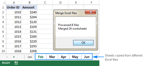
Depending on how many files you've selected, allow the macro a few seconds or minutes to process them. After the macro completes, it will notify you how many files have been processed and how many sheets have been merged: